Improve this page

Hydro-Geochemistry

Water and sediment geochemistry of the Cañete River Basin study area.

OUTLINE

This component of the project is looking at determinants of the water chemistry. The water chemistry is made up from geochemical contribution from the underlying geological units combined with input from anthropological activities (mining, agriculture, farming and domestic). This report will focus on an initial analysis of the data from the Cañete Basin water. The following outline and introduction has been reproduced from earlier reports. New analyses can be found in the discussion section.

The Cañete River basin is located in the central region of western Peru, in the provinces of Cañete and Yauyos in the department of Lima. The basin has a total area of 6,192 km2 (ANA report, 1970), with an average altitude of 3,686 masl and an average slope of around 12% (Apaclla Nalvarte, 2010). To the north and east the basin is bounded by the Mantaro River Basin, to the south by the San Juan (Chincha) River Basin, to the northwest by the Mala (and Omas) River Basin and its waters drain into the Pacific Ocean.

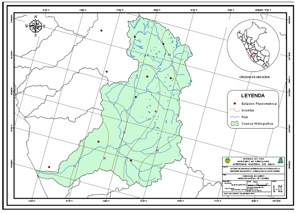Map of the Cañete River Basin (Apaclla Nalvarte, 2010)

The major river in the catchment is the Rio Cañete, which rises at the continental divide in the Ticlla and Pichahuarco mountain ranges of the Western Cordillera of the Andes (up to 5, 817 masl) and flows predominantly southwesterly towards the Pacific coast. The source is located at an altitude of 4,436 masl in Ticllaconcha Lake and is fed by glacial meltwater via a series of lagoons, and is sometimes referred to at this altitude as the Rio Caneje. It joins with the Rio Chichicocha to become the Rio Cañete in the high Andes (Apaclla Nalvarte, 2010). The Cañete River runs approximately 236km to the Pacific (Fransesconi. 2018) with an average slope of 2% (Ana report, 1970; Apaclla Nalvarte, 2010)

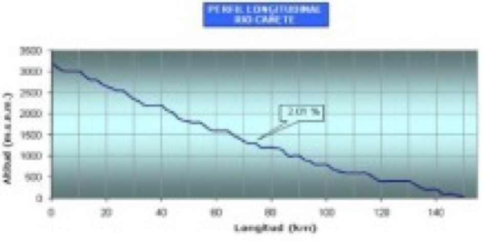Rio Cañete longitudinal profile (Apaclla Nalvarte, 2010)

The Cañete watershed can be divided into three distinct sections (Fransesconi. 2018): upper, middle and lower. The upper section of the watershed, which ranges between 4,000 to 5,800 m.a.s.l. contains the glaciers. The middle watershed is comprised by the area between 350 and 4,000 m.a.s.l., and the lower section has the smallest extent (4.6% of the watershed), and goes from sea level to 350 masl and is the focal area for agriculture in the basin.

Agriculture in the Cañete river basin below 500m is situated on the alluvial plain of the Cañete River and on the alluvial fans of Quilmaná and Conta and is reliant on waters from the river and its tributaries, both directly and via irrigation channels. Minor agricultural areas associated with settlements in the Yauyos Province above 2900m account for ~800 Ha of the total 22,457 Ha of agricultural land recorded in 2016 (INEI report 2016). Most of the agricultural land is given over to the production of maize and sweet potato, giving way to barley, potatoes and green beans in the Yauyos Province (INEI report 2016) and more subsistence farming.

The river flow is reliant on melting of glaciers in the source area and annual rains. The rainfall pattern in the Rio Cañete drainage basin indicates a sharp divide between the arid sub-tropics and tropics and the more humid temperate and puna life zones. Rains begin in November but the heaviest rainfalls in the basin are in February and March, and they vary between 20 mm and 160 mm/month. The least rainfalls are in July, and they vary between 10 mm in the humid temperate area and 0 mm in the basin’s lower arid area. Total annual rainfall in the Cañete River Basin varies between 1,000 mm and 200 mm, as shown in the Figure reproduced from appendix 2: hydrology of maximum floods in Cañete River, 2012.

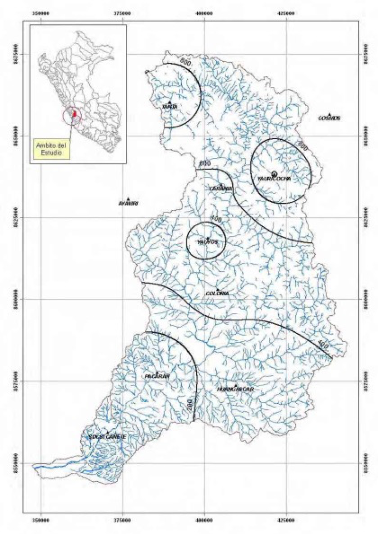Annual average rainfall patterns in the Rio Cañete (appendix 2: hydrology of maximum floods in Cañete River, 2012)

Maximum daily discharge rates reflect the variability between wetter and drier years (Apallca Nalvarte, 2010). The histogram shows the El Niño episodes falling during the same period as the discharge data (source) “Historical El Niño/La Niña episodes (1950–present)”. United States Climate Prediction Center), and there is some correlation between the highest daily discharge rates and these episodes. In a wetter year, possibly associated with El Niño events, rainfall may increase to 1700mm in the uplands.

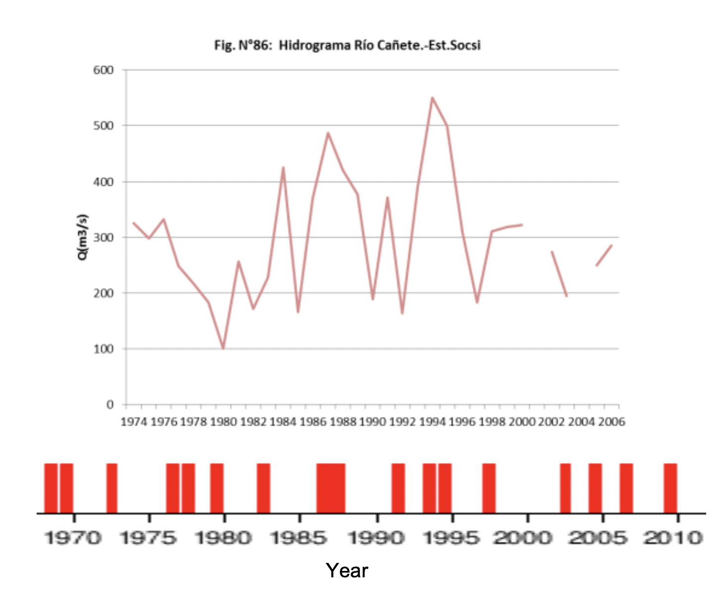Maximum daily discharge rates (Apallca Navafrte 2010) with El Niño episodes indicated by red bars (source) “Historical El Niño/La Niña episodes (1950–present)”. Note some correlation between the biggest peaks and strong ENSO.

Average monthly temperatures within the basin vary depending on seasonality and altitude. The report published by INRENA in 2002 shows temperature data for three weather stations in the catchment, at Cañete (150 masl), Pacarán (700 masl) and Yauyos (2290 masl) collected by SENAMI over an unspecified period. At the lower stations, annual temperatures average 20.7°C and 20.0°C with highs around 24°C in Feb/March and lows of 17-18°C in July/August. Temperature data for the station at Yauyos show very little seasonality, with an annual average of 17.6°C, and although it is slightly warmer in the months from September to December, there is very little deviation from the annual average throughout the year.

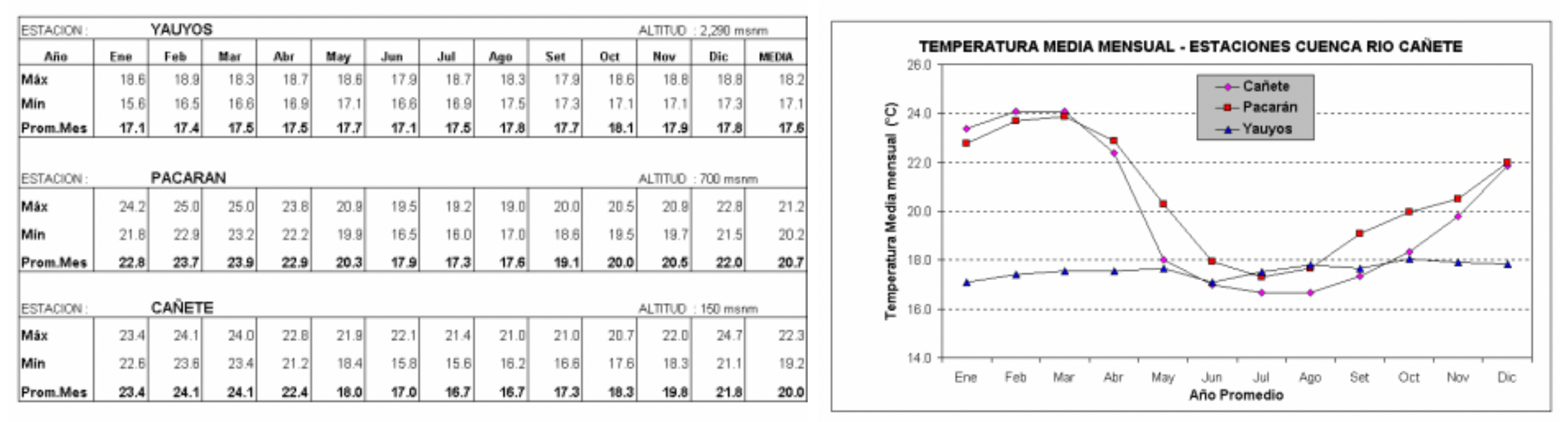Average monthly temperatures (°C) for three weather stations in the Cañete Valley, taken from INRENA (2002)

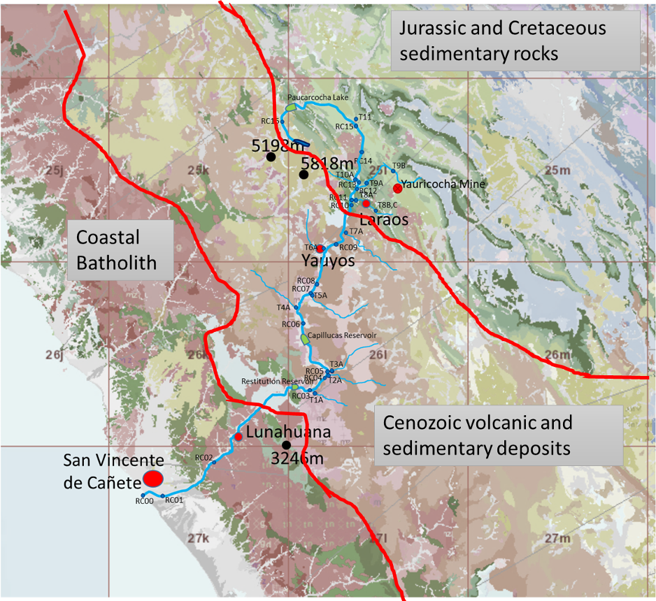
The Cañete Basin is underlain by a large Mesozoic sedimentary basin, filled with both marine and continental lithologies; predominantly fine-grained sedimentary rocks with volcanic intercalations (andesites, dacites), limestones, sandstones, shales, etc. These have been heavily deformed by the intrusion of synorogenic batholiths (Coastal Belt) and continental scale deformation (forming the Western Cordillera), as a result of subduction of the Nazca Plate under the South American Plate, leading to formation of the Andes and the concomitant development of various structures such as faults and folds in the Andean foreland (see cross section above). These deposits are overlain unconformably by Cenozoic rocks associated with evolution of the active and topographically elevated volcanic arc, in addition to igneous intrusions of granitoid composition and volcanic effusions that partially or totally cover the oldest structures and rocks.

The age of the rocks in the basin range from the Lower Jurassic to recent Quaternary with the older rocks cropping out in belts running parallel to the Andean Cordillera in the upper parts of the basin (see geological map (ANA “Cuenca del Rio Cañete” report). The Cañete River flows from the headwaters in Mesozoic sedimentary rocks, through the fold and thrust belt of the Western Cordillera, down through the Coastal Batholith and associated volcanics in the central area and finally through a thick alluvial-fluvial sequence cutting down to the coastal plain and out to the sea.

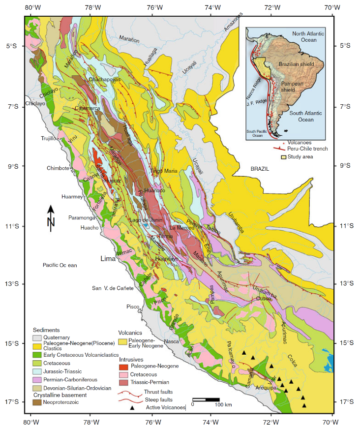Generalized geological map of the Peruvian Andes showing main lithologies and major thrust faults. Thrust faults mark the base of the eastern escarpment of the Eastern Cordillera. The Coast Batholith outcrops along the western escarpment of the Western Cordillera (Gonzales & Pfiffner, 2011)

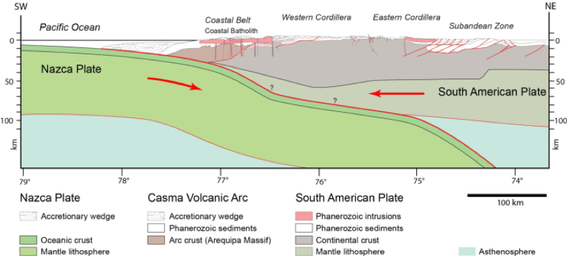General cross-section showing the geometry of the plate boundary in the subduction zone and the crustal structure of the Andes (Pfiffner & Gonzales, 2013)

The chemistry of water is affected by the rock units it is flowing over and through. This will give the river a unique chemistry; each tributary adds its unique chemistry to the main channel, which becomes summative downstream. Different trace metal chemical species will behave differently depending on the dominant major element composition of the water, the pH, temperature, altitude, and residence time of the water in the system. The effect of any one tributary on the main channel water chemistry is moderated by the relative flux of the tributary compared to the flow volume in the main channel. In addition, the water chemistry will be affected seasonally by changes in precipitation affecting runoff and groundwater flux, as well as variability in the amount and timing of water extracted for irrigation/hydrothermal energy production etc or released from reservoirs upstream.

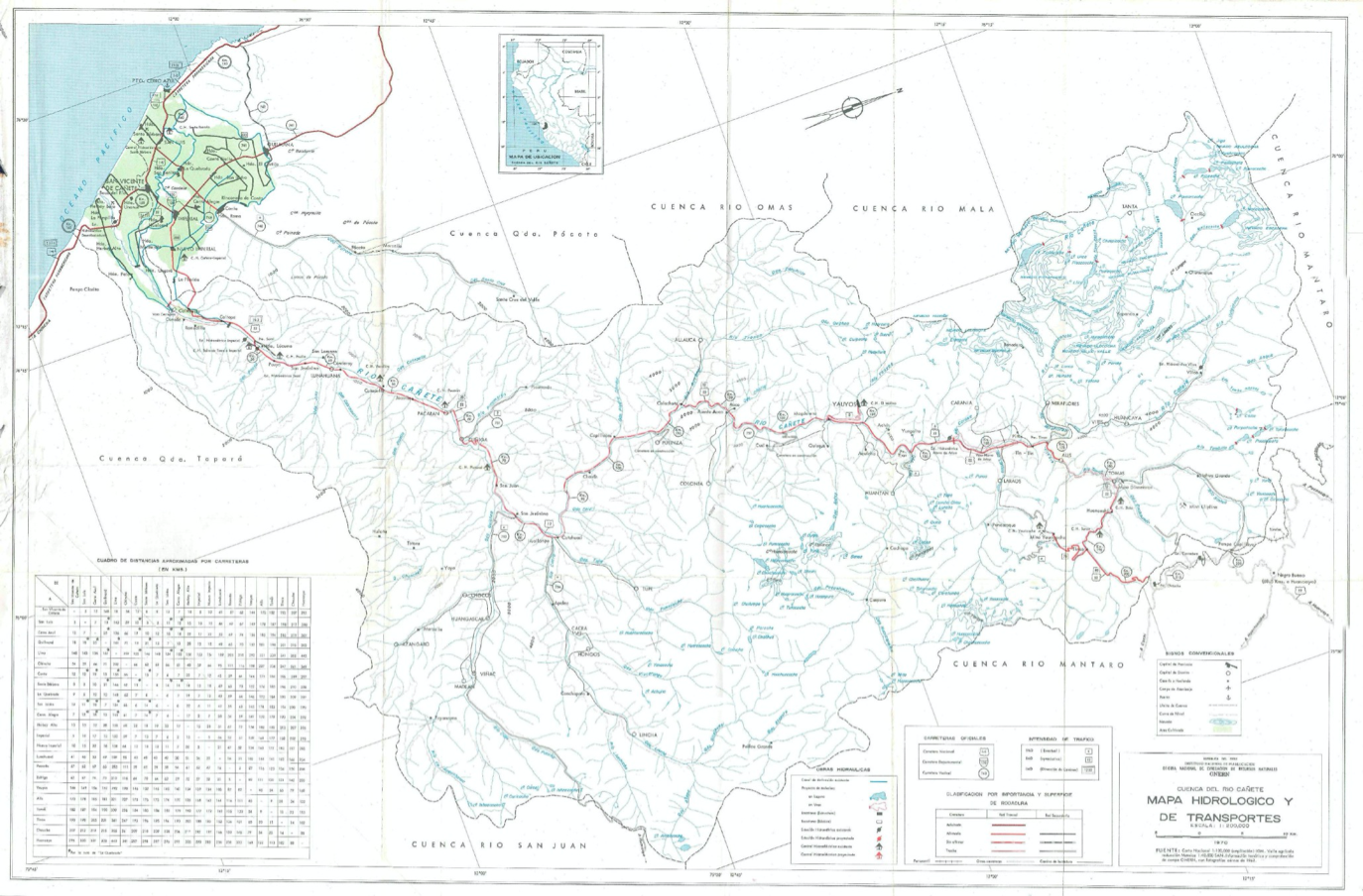Hydrographic map of the Cañete Basin (from ANA “Cuenca del Rio Cañete” report, 1970)

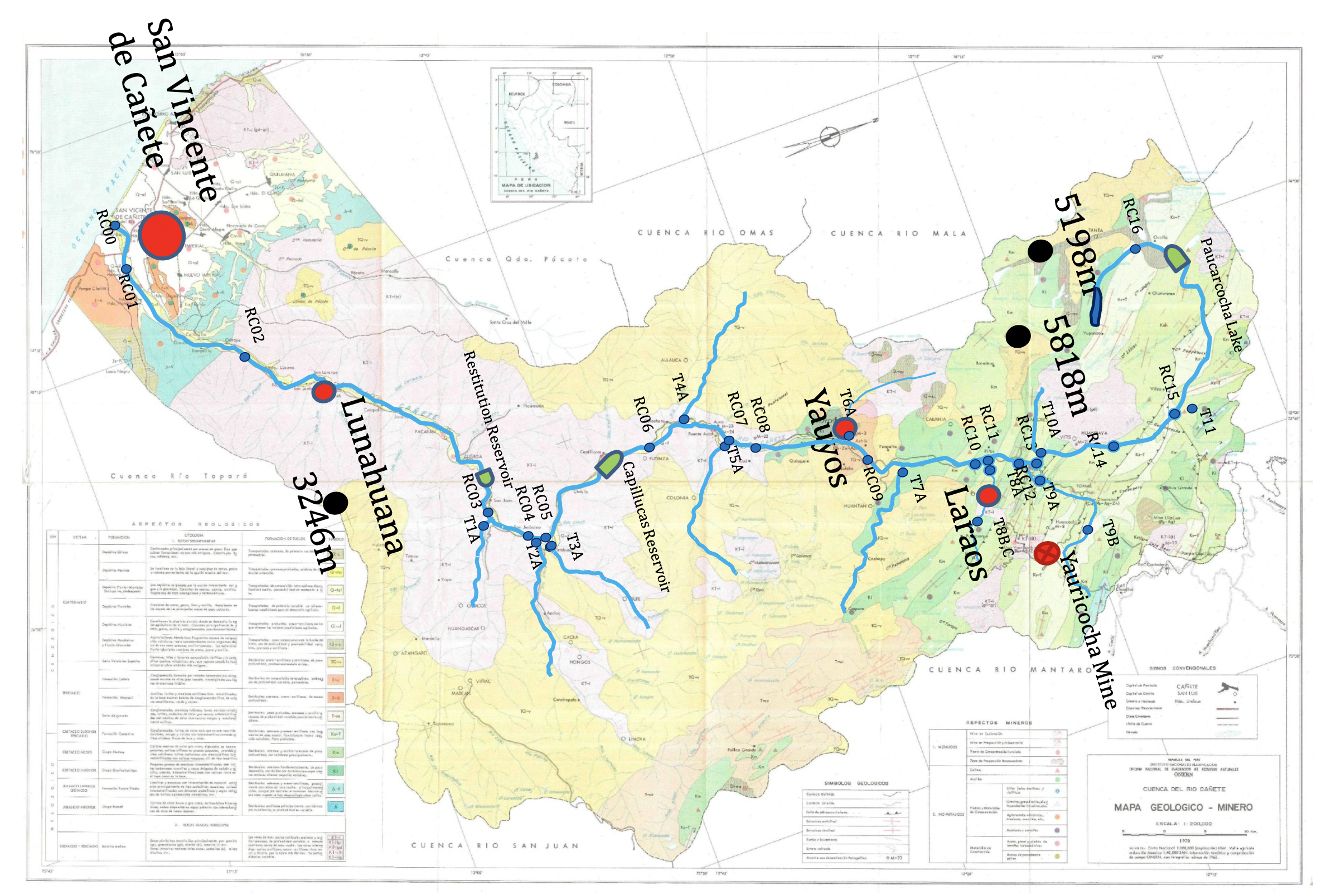Geological map of the Cañete Basin (from ANA “Cuenca del Rio Cañete” report, 1970) with sample network superimposed

AIMS AND OBJECTIVES

The aim is to investigate endmember determinants for river water chemistry in the Cañete River. Field expeditions will collect paired water and riverbed sediment samples. Rock units are naturally heterogeneous, but the fluvial processes act to homogenise the clastic material from the catchment. Because both the particulate load and chemical signal from the river water are naturally additive as one goes down stream, samples need to be taken from sites ranging from the upper basin to the coast and from the tributaries to understand the proportional chemical contribution from all areas. Modelling will allow determination of the various chemical contributors to the water chemistry. In addition, there are some interesting and less well studied geological units within the catchment. More detailed fieldwork will allow us to determine the environment of deposition and how this changed through geological time. Understanding changes in sedimentary depositional environments ultimately helps us to understand large scale tectonic and climatic processes in the past.

MATERIALS AND METHODS

Water Sampling

Water samples were collected from selected 32 sites in the Cañete River and its tributaries (see table and site map). Sampling trips are planned to represent the river in both dry and wet seasons. So far, samples have been collected in July and November in 2019. More sets will be collected to look at seasonal variability. Filtered water samples were collected for inorganic tests including metals, trace metals and anions. Unfiltered samples were collected for alkalinity measurements and for a few samples to assess suspended:dissolved metal species.

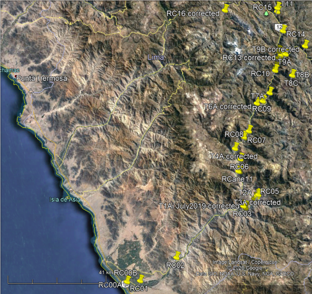Site network. Image: Google Earth

Site Code	Site Number	Site Name
RC00B	1	Canete estuary - Herbay Bajo
RC01	2	Canete - Herbay Alto
RC02	3	Rio Canete - Bocatoma Canete
RCO3	4	Canete - Llangas Tambo
T1aii	5	Vinac. Vinac bajo
RC04	6	Canete, below Huallampi
T2a	7	Lincha. Lower Lincha, Puente Cacra
RC05	8	Canete. Below Catahuasi
T3a	9	Tupe. Below Catahuasi. Tupe sector.
RC06	10	Canete. Calachota
T4a	11	Calachota. Above Calachota
RC07	12	Canete. Above Puente Auco
T5a	13	Colonia (was Auco). Above Puente Auco
RC08	14	Canete. Below Yauyos. Puente Huayo.
T6a	15	Yauyos. Below Yauyos (above Magdalena)
RC09	16	Canete. Huantan. Puente Aquicha.
T7a	17	Huantan. Below Huantan
RC10	18	Canete. Below HEP plant
RC11	19	Canete. Above HEP plant, Villa de Arma
T8a	20	Laraos. Below Laraos
T8b	21	Laraos. Above Laraos, Puente Union
T8C	21.5	Laraos. Manantial de Laraous. A spring with beautiful plants.
RC12	22	Canete. Villa da Alma, below Tinco Alis
T9a	23	Alis. Below Alis
T9b	24	Alis. Headwater site. Above Huancachi
RC13	25	Canete, P. Acomachay, below confluence.
T10a	26	Miraflores, P.Chunque - near confluence
RC14	27	Canete. Above Huancaya
RC15	28	Canete. P.Vitcos. Below Rio Vilca confluence
T11a	29	Vilca- near confluence.
RC16	30	Above Tanta

Composite water samples are collected into a prewashed polyethylene bottle at each site. Each bottle is held to allow collection of water directly from the upstream flow of the river. Samples are stored in a cool box with ice packs and transferred to a laboratory refrigerator kept at 4ºC at the end of the day. Additional water samples are collected into 50 ml test tubes and 500 ml pre-washed HDPE bottles for sending to commercial labs for different chemical analyses. A subset of the sample is filtered at the site to remove suspended particles (which are also retained for analysis). This reduces the possibility of alterations to the “original” water chemistry subsequently taking place in the bottle.

On-site analysis for pH, temperature, dissolved oxygen, electrical conductivity (specific conductivity), oxidation reduction potential and total dissolved solids is recorded for each sample. Environmental data including atmospheric pressure and temperature, river water flow rate, and depth and approximate width of the rivers are recorded. River flow rate, width and depth are used to calculate discharge and chemical flux. Each site is photographed and anthropogenic activities and natural features noted for context.

Sediment samples are collected from the river bank or bed, wherever the sediment has the smallest grain size. Sediment with smaller grain size is better sorted and more homogeneous than those with a larger grain size and so gives a better representation of the different lithologies exposed in the catchment area. Both sedimentary and water samples are then analysed for a suite of major and trace elements and minerals at labs in Peru and in Cambridge.

Alkalinity (mg/l of calcium carbonate) is measured using a digital Hach titrator on unfiltered samples within 24 hours of collection (~see Hach document DOC316.53.01166 for details). Titration is conducted in two steps using 1.6N and/or 0.16N H2SO4, and Phenolpthalein and Bromcresol / Methyl powders as indicators to ascertain the Phenolpthalein end point (pH 8.3) and the total alkalinity (pH 4.5). Phenolpthalein is first added to 100ml of unfiltered water in a clean 250ml glass flask. If the sample colour turns pink, acid is added dropwise from the titrator to the water sample until a colour change of pink to colourless indicating the sample now has a pH 8.3. The number of digits added is recorded. Once the sample has turned colourless, or if it was already colourless on initial addition of the Phenolpthalein, Bromcresol / Methyl is added to the sample. The sample will turn green. More acid is added until the sample reaches pH 4.5 when the colour changes to pink. The total number of digits used is now recorded. If the sample is pink on initial addition of the Bromcresol / Methyl, the sample has no alkalinity (i.e. no capacity to buffer addition of H+ ions) and no titration is conducted. If the sample is known to have a low pH, the 0.16N H2SO4 is used. For samples with mid range pH, the titration should be started with the 1.6N H2SO4. If the samples turn pink very quickly, the acid cartridge should be swapped to 0.16N and the titration repeated.

Sample volumes and digit multipliers. In order to calculate alkalinity as mg/l CaCO3, a digital multiplier (dependent on the normality of the acid) is applied to the digital counts. Select a range in Table 1, then read across the table row to find the digital multiplier for this test. Use the digit multiplier to calculate the concentration in the test procedure.

Examples:

A 100-mL sample was titrated with the 0.1600 N Sulfuric Acid Titration Cartridge and the counter showed 40 digits. The concentration is 40 digits x 0.1 = 4 mg/l as CaCO3 total alkalinity.

A 100-ml sample was titrated with the 1.600 N Sulfuric Acid Titration Cartridge and the counter showed 250 digits to the first end point. The concentration is 250 digits x 1 = 250 mg/l as CaCO3 Phenolpthalein alkalinity (at pH 8.3). This would allow you to calculate the concentration of hydroxide and half the total amount of carbonate ions in the sample (Table 2). One would then need to continue the titration to the second end point to calculate the total alkalinity.

Table 1 Sample volumes and digit multipliers

Range (mg/l as CaCO3)	Sample volume (ml)	Titration cartridge	Digit multiplier
10–40	100	0.1600 N H2SO4	0.1
40–160	25	0.1600 N H2SO4	0.4
100–400	100	1.600 N H2SO4	1
200–800	50	1.600 N H2SO4	2
500–2000	20	1.600 N H2SO4	5
1000–4000	10	1.600 N H2SO4	10

The dominant ions involved in the alkalinity can be calculated using table 2:

Table 2 Alkalinity relationships

Row	Titration result	Hydroxide alkalinity	Carbonate alkalinity	Bicarbonate alkalinity
1	P alkalinity = 0	0	0	= Total alkalinity
2	P alkalinity = Total alkalinity	Total alkalinity	0	0
3	P alkalinity is less than ½ of Total alkalinity	0	= P alkalinity × 2	= Total alkalinity – (P alkalinity × 2)
4	P alkalinity = ½ Total alkalinity	0	= Total alkalinity	0
5	P alkalinity is more than ½ Total alkalinity	= (P alkalinity × 2) – Total alkalinity	= (Total alkalinity – P alkalinity) × 2	0

To date, no Cañete samples have any hydroxide or carbonate alkalinity. All alkalinity is attributable to bicarbonate ions (see results below).

Water sampling protocols were developed following the guidelines from WHO, United States Environmental Protection Agency (USEPA) and ANA of Peru. For full details of sample collection protocols – refer to the field sampling manual in the appendix. This report will focus on initial analysis of the water data only.

Sample analysis in laboratories

Inorganic analyses were conducted by Inductively coupled plasma mass spectrometry (ICP-MS), Inductively coupled plasma optical emission spectroscopy (ICP-OES) and Ion chromatography (IC) in the SGS Laboratory (Lima, Peru – Nov 2019 data) and at the Pontificia Universidad Católica del Peru labs (July 2019 data).

Sample analysis for organics was carried out using Gas Chromatography (GC) with packed column and electron capture detector, and High-performance liquid chromatography (HPLC) with diode array detector. Microbiological analysis was carried out with Multiple-Tube Fermentation Technique for Total and Thermal Coliform and Escherichia coli.

All tests were carried out in quality-controlled labs following standard procedures.

DISCUSSION AND FUTURE WORK

Initial analyses of the Cañete River water and sediment confirms that in general the water in the river is of a very high standard with very little contamination (see report 2). The chemistry of the river, and its sediments is dominantly controlled by the geology, with varying contribution from hydrothermal waters and minor anthropogenic factors predominantly affecting the tributaries. The significant proportion of Jurassic and Cretaceous carbonate rocks is reflected in the pH, alkalinity and major ions. The pH is slightly acidic (in the dry season av. 6.03) to slightly alkaline (in the wet season av. 8.58) pH (fig. 1). This is in line with previously reported pH for the river system (INEI 2016).

INEI 2016 Cañete River pH data from the surface waters of the bay

	Mín.	Máx.
2006	7.41	8.29
2007	7.03	7.89
2008	6.61	7.91
2009
2010	6.73	8.19
2011	7.83	8.05
2012	7.46	8.43
2013	7.27	8.6
2014	7.72	8.49
AVERAGE	7.26	8.23

The range in pH values throughout the year is not simply down to dilution, if this were the case the wetter season should record values closer to pH 7 but instead they record greater alkaline values. Greater or lesser discharge and the relative amount of H2O in the system cannot change pH from acidic (<7) to alkaline (>7) but only drive it towards neutrality (pH 7). The change in pH suggests it is not merely a dilution or concentration of chemicals during greater or lower flow. Instead, the data show increased levels of bicarbonate ions during the rainy season (immediate response of increased weathering in the limestone catchment). Whilst, in contrast, dilution of sulfate ions in the wet season coupled with the relatively slower but constant release of sulfate through aqueous weathering of pyrite throughout the year (Williamson, M. A. and Rimstidt, J. D., 1994; Hercod et al 1998) creates relatively higher levels of sulfate in the dry season (fig 2). Rates of silicate weathering are at least ten times slower than sulfide weathering (Torres et al, 2017) and do not dominate the anion trends.

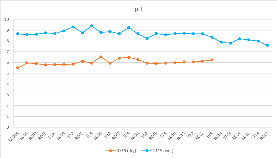pH in the dry and wet season along the Cañete river system and its tributaries.

In absolute terms, bicarbonate is the dominant anion in the main channel throughout the year, with an average of 52% in the dry season and 55% in the wet season, followed by sulfate and chlorite respectively (figs. 2 and 3). Note that sulfate concentrations are higher in the dry season.

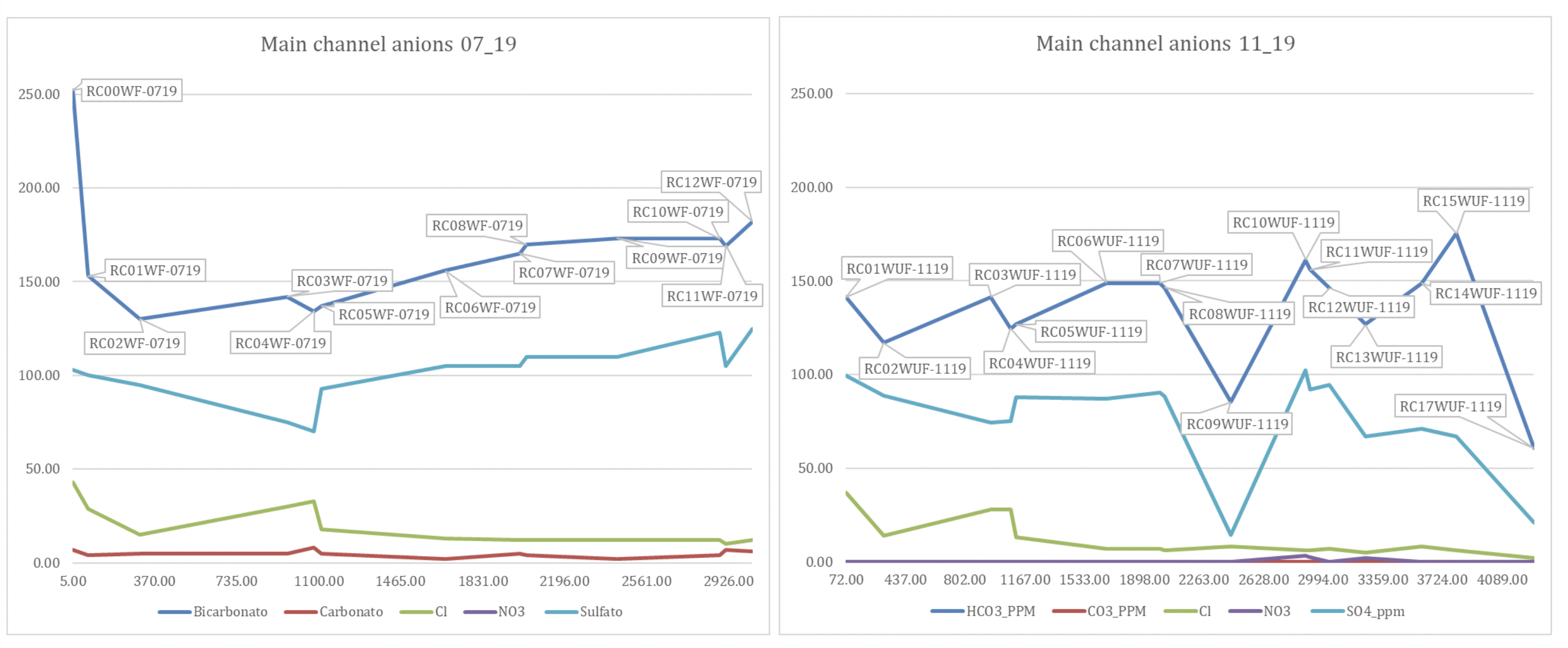Water Anion .chemistry plotted against altitude for the main channel only, a) July 2019 (dry), b) November 2019 ~(wet).

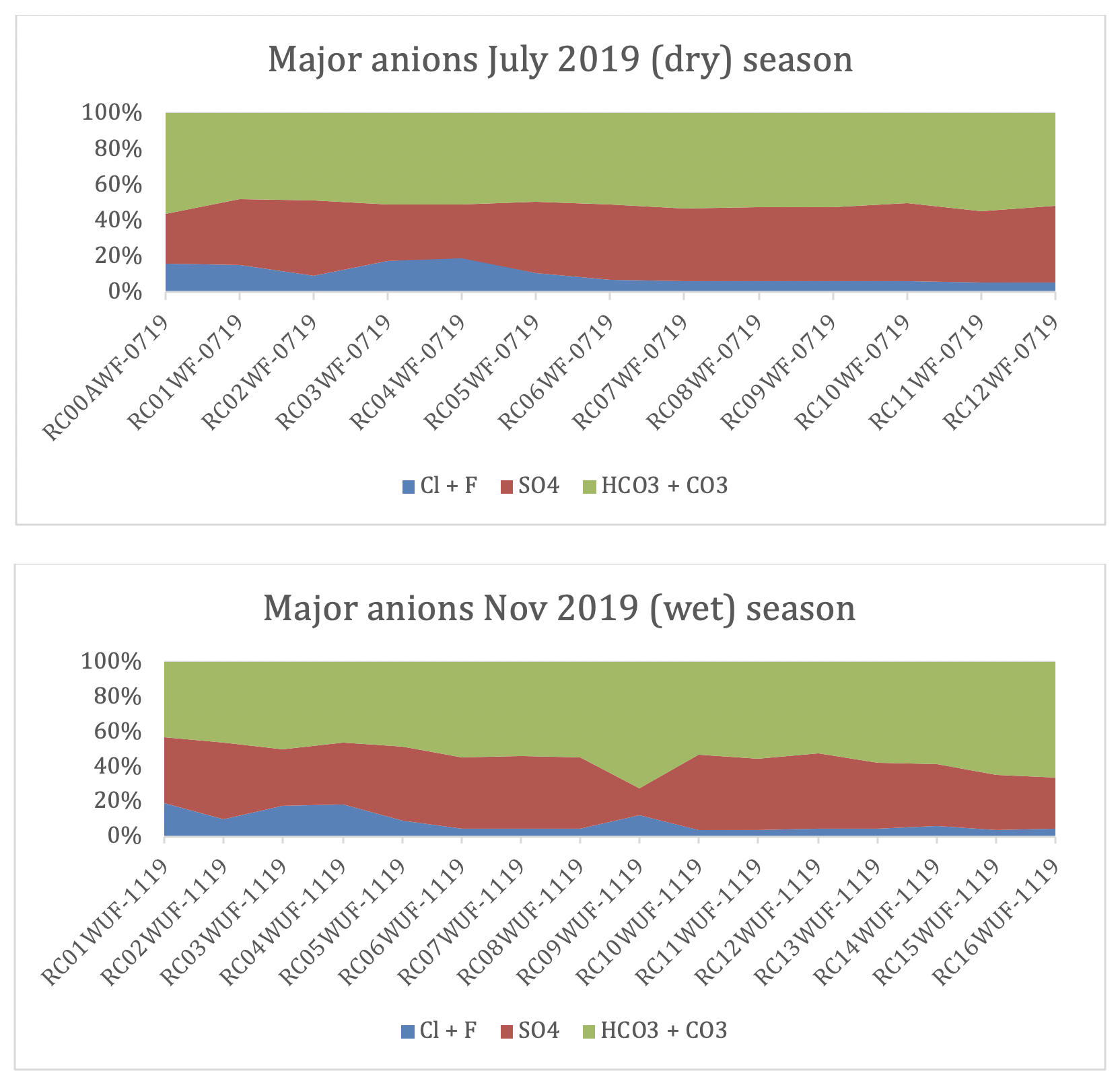Percentage of major anions in the dry and wet season along the Cañete main river system. Note the relative increase in chlorine downstream. This is probably a combination of increasing proximity to the ocean and anthropogenic factors.

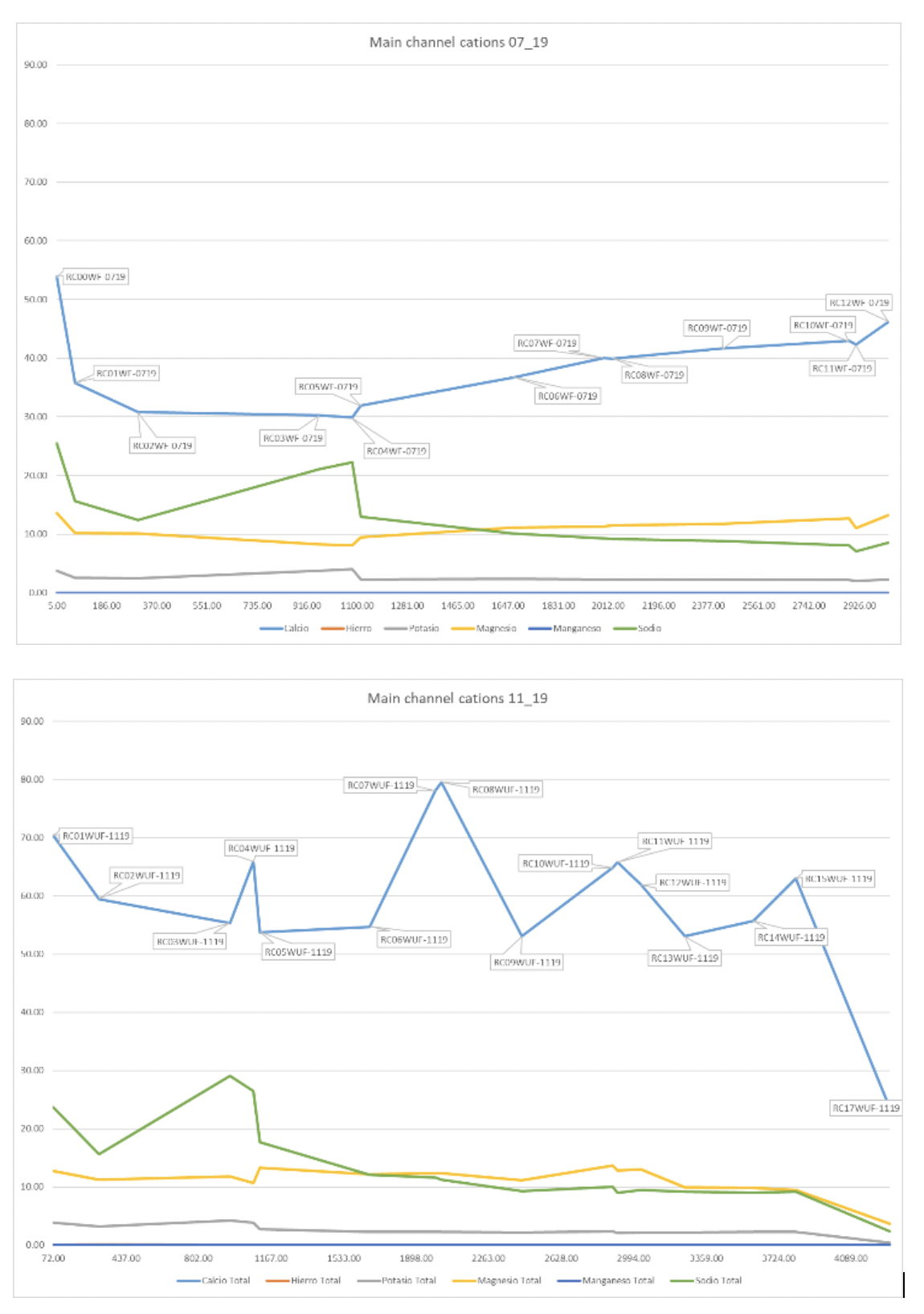Major element cations chemistry plotted against altitude for the main channel only, a) July 2019 dry, b) November 2019 wet. You can clearly see the effects of the tributaries on the mainstream chemistry when there is more flow in November.

Cation chemistry is dominated by calcium throughout the year with substantially higher concentrations in the wet season than the dry and clearly heavily influenced by incoming tributaries, whilst other cations show fairly consistent concentrations across the two seasons (Fig. 4). Proportionally, calcium is the dominant cation (Fig. 5); averaging 54% in the dry season and 68% in the wet season, although there is more variability within the wet season data (st dev = 6.8%). Sodium increases in absolute concentration downstream as the drainage weathers increasingly more silicate rich rocks, diluting the calcium signal, and samples are also closer to the chemical influence of the sea.

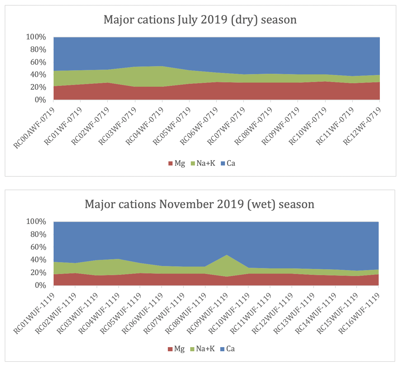percentage of major cations in the dry and wet season along the Cañete main river system. Note the relative increase in sodium downstream. This is probably a combination of increasing proximity to the ocean. RC09 has elevated sodium and chlorine (fig. 3) which could reflect addition of briney groundwater.

The tributaries are more variable in their major cation and anion chemistry, reflecting a less diluted signal from the local geology due to the lower flow volumes and shorter distance travelled from source.

The relative proportions of major cations and anions can be plotted on a Piper diagram (Piper, 1944) this allows a visual comparison of the variation in water chemistry, and the assigning of hydrochemical facies within the catchment.

Piper or trilinear plots:

Variations in major ion water chemistry are plotted using a variety of different geochemical plots. Piper diagrams or Stiff plots, for example, are highly visual representations of the major ions in fluvial samples and allow for quick grouping of different water bodies and to identify shifts in water chemistry. The Piper or trilinear plot (Piper, 1944) is especially useful for classifying hydrochemical facies.

A piper plot is comprised of three components (Fig. 6): a ternary diagram in the lower left representing cations (magnesium, calcium, and sodium plus potassium), a ternary diagram in the lower right representing anions (chloride, sulfate, and carbonate plus bicarbonate), and a diamond plot in the middle, which is a matrix transformation of the two ternary diagrams. Cations and anions are converted to meq/L and normalized (sum of cations = 100 and sum of anions = 100), so the relative concentrations are on a percentage basis.

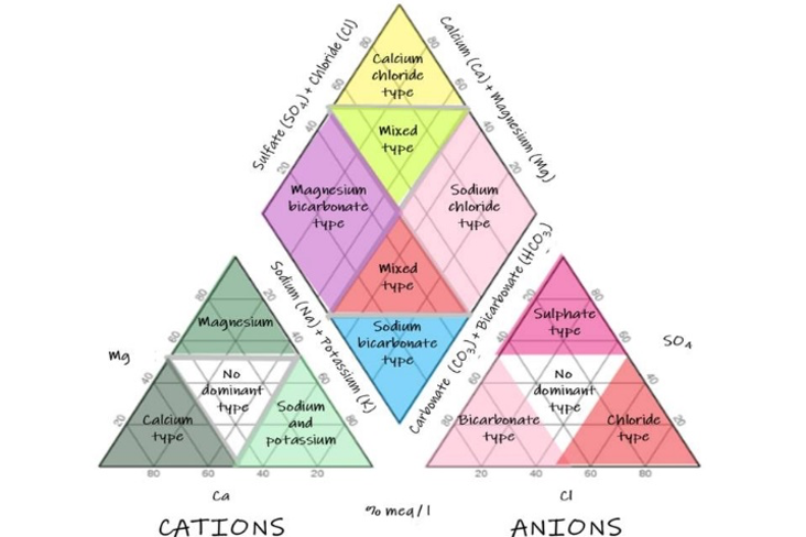Diagram showing the elements of a Piper diagram. Depending on the dominant cations and anions in any one sample the hydrochemical facies will have slightly different names (Magnesium bicarbonate vs Calcium bicarbonate for example).

In the Cañete river system the dominant cations are calcium and sodium, with bicarbonate and sulfate dominating the anions. Therefore, samples in the top quadrant are calcium sulfate waters, which are typical of pyrite oxidation coupled with carbonate weathering (Hercod et al 1998), acid mine drainage or gypsum ground water. Samples in the left quadrant are calcium bicarbonate waters, which are typical of shallow fresh ground water. Samples in the right quadrant are sodium chloride waters, which are typical of marine and deep ancient ground water (brine). Samples in the bottom quadrant are sodium bicarbonate waters, which are typical of deep ground water influenced by ion exchange.

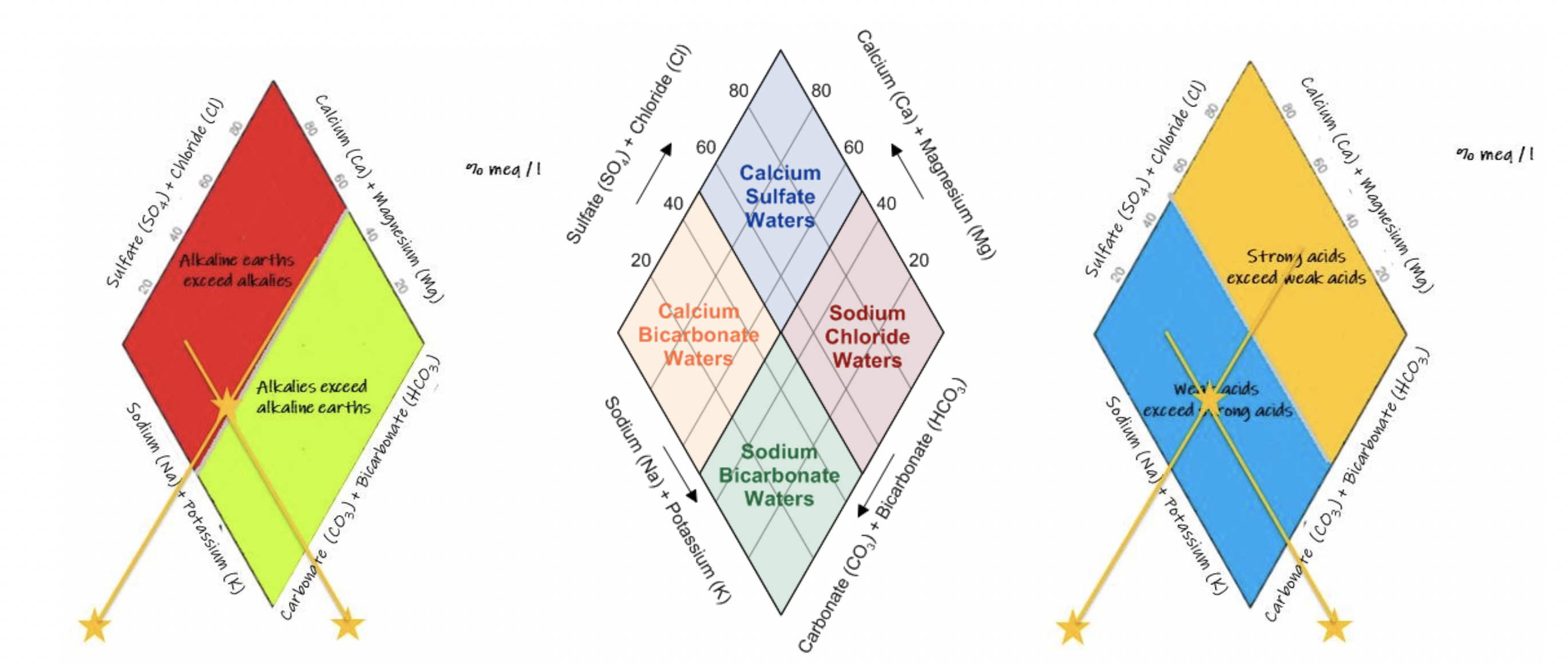Diamond plots showing the different fields for hydrochemical facies, weak vs strong acids and alklaies vs alkaline earths

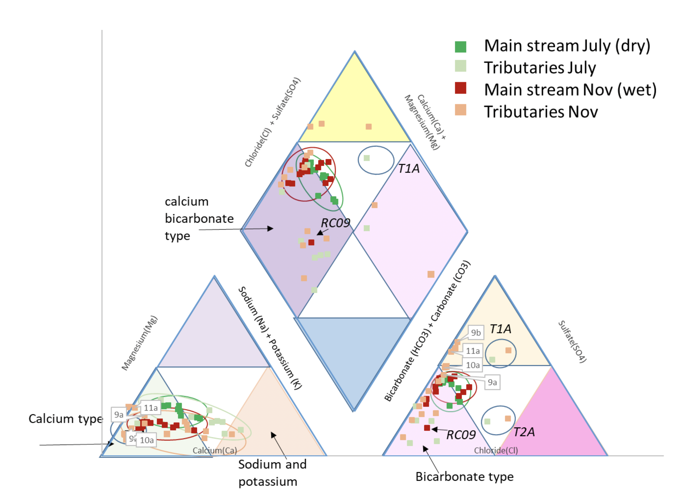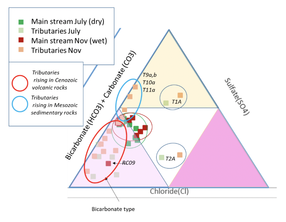
Piper diagram for the Cañete River and its tributaries.

Using figure 8 it is now possible to start to investigate more closely the hydrochemical facies of the Cañete River and its tributaries. The diamond plot shows that the main channel and the majority of the tributary waters are dominantly Calcium Bicarbonate to mixed type, and alkaline earth dominant. The chemistry is consistent with weak acids dominating over stronger acids. This does not mean the water is acidic but reflects the relative reactivity of the dominant anions.

It is useful to consider the cation (fig. 9) and anion (fig. 11) triangular plots in a little more detail. The cation data appears to show linear trends in the mainstream (although the November data contains relatively more calcium/less magnesium than the dry season), with the tributaries perhaps not all following this trend. On investigation this trend proves to be broadly true, with a proportional increase in sodium (and potassium) in samples downstream (RH figure). The Left hand figure shows the tributary chemistry for the two seasons, subdivided by the geology they flow over (Fig. 12). Tributaries T8, T9, T10 and T11 all arise in the Jurassic and Cretaceous limestone in the upper part of the basin and their chemistry is dominantly “calcium type”. The other tributaries flow over and through the volcanic rocks of Cenozoic age and are of sodium (and potassium) type. There are no tributaries flowing through the older Coastal Batholith. The Coastal Batholith is dominated by silicic intrusive rocks, and as these are relatively resistant to chemical weathering, the rocks here would not be expected to contribute much to the river chemistry (figs. 10 and 12).

The mainstream anions (fig. 11) cluster for both seasons as bicarbonate (to mixed) type. The volcanic tributaries are dominated by bicarbonate type, whilst the limestone tributaries show a trend towards sulfate type. This is consistent with a coupling between pyrite oxidation and calcite weathering in the colder upper catchment (Hercod et al., 1998).

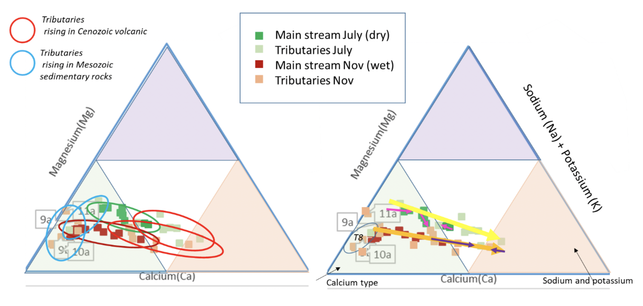Cation triangular plots for Cañete River and tributaries. LH: showing the different chemical types for the tributaries arising over different geology; RH showing the trend downstream from calcium type to sodium type waters.

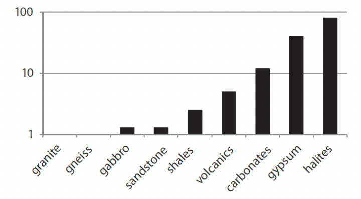Compilation of rock dissolution rates by Gislason, S. R. et al., 2011.

Anion triangular plots for Cañete River and its tributaries, showing the clustering of the mainstream samples and the different chemical types for the tributaries arising over different geology

A simplified geological map (INGEMMET 2017 basemap) and overlay of sample sites showing which tributaries lie within which geological units.

CONCLUSION

The initial analysis of water samples suggest the main Cañete River is chemically very clean with some unique chemical signals coming in from tributaries largely dictated by the geological units they flow over and through. The next steps are to model the quantitative effect of the tributaries in both wetter and drier seasons, using the chemistry and the flux. We will analysis and relate the sediment chemistry to the water chemistry, and in particular look at hydraulic sorting and the residence times for trace metals. We will further investigate the quantitative effect of the different rock types, and chemical weathering of these, on the water quality in different sections of the river.

REFERENCES

Mesozoic–Cenozoic Evolution of the Western Margin of South America: Case Study of the Peruvian Andes. O. Adrian Pfiffner and Laura Gonzalez. Geosciences 2013, 3, 262-310

Morphologic evolution of the Central Andes of Peru. Laura Gonzalez and O. Adrian Pfiffner. Int. J. Earth Sci. 2012, 101, 307–321

Cuenca del Rio Cañete, ANA Report 1970.

Hydrology Of Maximum Floods In Cañete River - Appendix 2. Project of the protection of flood plain and vulnerable rural population against floods in the republic of Peru. Japan International Cooperation Agency and Ministerio de Agricultura de Peru. 2012

Compendio Estadístico Lima Provincias 2016 (Statistical compendium of Lima provinces, 2016). Instituto Nacional de Estadistica e Informatica (INEI).

Estudio de máximas avenidas en las cuencas de la zona centro de la vertiente del Pacífico. Informe final. ANA report: Apaclla Nalvarte, 2010

“Historical El Niño/La Niña episodes (1950–present)”. United States Climate Prediction Center https://origin.cpc.ncep.noaa.gov/products/analysis_monitoring/ensostuff/ONI_v5.php

Modelling for Management: A Case Study of the Cañete Watershed, Peru. Wendy Francesconi, Natalia Uribe, Jefferson Valencia and Marcela Quintero, 2018. In Andean Hydrogeology, Chapter 4, pg 84-101.

Compendio Estadístico Lima Provincias 2016. INEI 2016

Ni 43-101 Technical report on the Yauricocha Mine, Yauyos Province, Peru, 2015. Donald E. Hulse, P.E., Thomas C. Matthews, and Deepak Malhotra, Gustavson Associates for Sierra Metals, Inc.

Piper, A.M., 1944. A graphic procedure in the geochemical interpretation of water-analyses. Eos, Transactions American Geophysical Union, 25(6), pp.914–928.

Williamson, M. A. and Rimstidt, J. D., 1994. The kinetics and electrochemical rate-determining step of aqueous pyrite oxidation. Geochimica et Cosmochimica Acta, Vol. 58. No. 24, pp. 5443-5454.

INRENA report 2002. Evaluación y Ordenamiento de los Recursos Hídricos de la Cuenca del río Cañete.

Hercod, D. J., Brady, P. V. and Gregory, R.T., 1998. Catchment-scale coupling between pyrite oxidation and calcite weathering. Chemical Geology, 151, 259–276.

Gislason, S. R. et al., 2011. Silicate Rock Weathering and the Global Carbon Cycle, pp. 84–103. John Wiley & Sons, Ltd.